
Digit Recognition using LeNet
Some Cool Convolutional Neural Network in Action.
CONTEXT
-
MNIST (“Modified National Institute of Standards and Technology”) is the de facto “hello world” dataset of computer vision. Since its release in 1999, this classic dataset of handwritten images has served as the basis for benchmarking classification algorithms. As new machine learning techniques emerge, MNIST remains a reliable resource for researchers and learners alike.
-
The data files train.csv and test.csv contain gray-scale images of hand-drawn digits, from zero through nine. Each image is 28 pixels in height and 28 pixels in width, for a total of 784 pixels in total. This pixel-value is an integer between 0 and 255, inclusive.
-
The test data set, (test.csv), is the same as the training set, except that it does not contain the “label” column.
AIM
- LeNet is Used to design a digit recognition Algorithm that correctly classifies the digits 0 to 9.
- Simple and efficient system with high accuracy.
Importing Necessary Libraries
import pandas as pd
import numpy as np
import random
import seaborn as sns
import matplotlib.pyplot as plt
import tensorflow as tf
from tensorflow.keras import models
from tensorflow.keras import layers
from tensorflow.keras.utils import to_categorical
sns.set_style("darkgrid")
Reading CSV
#Importing Data
train = pd.read_csv("../input/digit-recognizer/train.csv")
test = pd.read_csv("../input/digit-recognizer/test.csv")
#Separating labels and predictors
X = train.drop("label",axis=1)
y = train[["label"]]
Preprocessing Step
def preprocess_data(X,test,y):

    #Reshaping
    X = np.array(X).reshape(X.shape[0],28,28,1)
    test = np.array(test).reshape(test.shape[0],28,28,1)

    #To categorical
    y = to_categorical(y)

    #Rescaling
    X    = X/255.0
    test = test/255.0
    return(X,test,y)
#Applying the function
X,test,y = preprocess_data(X,test,y)
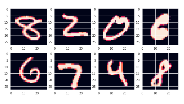
Visualising the MNIST Data
plt.figure(figsize=(10,5))
for i in range(1,9):
  ind = random.randint(0, len(X))
  plt.subplot(2,4,i)
  plt.imshow(tf.squeeze(X[ind]))
Data Splitting
#Generating random integers
val_size = int(X.shape[0]*0.2)
val_ind = random.sample(range(1,X.shape[0]),val_size)
#Validation Data
x_val = X[val_ind]
y_val = y[val_ind]
#Training Data
x_train = np.delete(X, val_ind, axis = 0)
y_train = np.delete(y, val_ind, axis = 0)
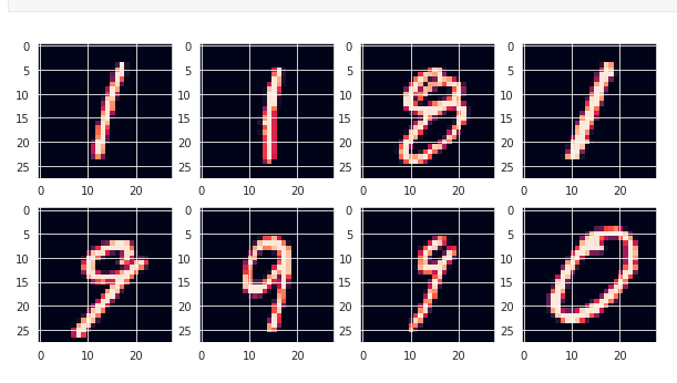
Visualising the Training data
#Train Data
plt.figure(figsize=(10,5))
for i in range(8):
  ind = random.randint(0, len(x_train))
  plt.subplot(240+1+i)
  plt.imshow(tf.squeeze(x_train[ind]))
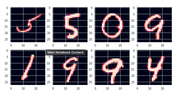
Visualising the Validation data
#Validation Data
plt.figure(figsize=(10,5))
for i in range(8):
  ind = random.randint(0, len(x_val))
  plt.subplot(240+1+i)
  plt.imshow(tf.squeeze(x_val[ind]))
LeNet Architecture
sizes = [277942,496048,21638,]
labels = ['Active', 'Recovered', 'Deaths']
explode = [0.05,0.05,0.05]
plt.figure(figsize=(12,8))
plt.pie(x=sizes,labels=labels,startangle=9,colors=['#66b3ff','green','red'],autopct="%1.1f%%",explode=explode,shadow=True);
plt.title("Covid-19 India Cases",fontsize=20);
centre_circle = plt.Circle((0,0),0.70,fc='white')
fig = plt.gcf()
fig.gca().add_artist(centre_circle);
plt.tight_layout()
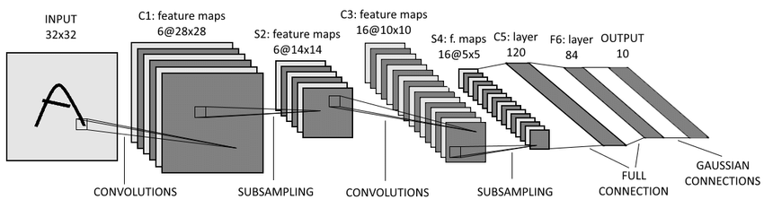
Architecture Explained
-
In the figure above, The First layer is a input layer followed by a convolutions, pooling and fully connected layers.
-
The input is images of size 28 × 28.
-
C1 is the first convolutional layer with 6 convolution kernels of size 5×5. Followed by the pooling layer that outputs 6 channels of 14 × 14 images. The pooling is of size 2 × 2.
-
C2 is a convolutional layer with 16 convolution kernels of size 5 × 5. Hence, the output of this layer is 16 feature images of size 10 × 10. Followed by a pooling layer with a pooling size of 2 × 2. Hence, the dimension of images through this layer is halved, it outputs 16 feature images of size 5 × 5.
-
F3 is the fully connected layer with 120 neurons. Since the inputs of this layer have the same size as the kernel, then the output size of this layer is 1 × 1. The number of channels in output equals the channel number of kernels, which is 120. Hence the output of this layer is 120 feature images of size 1 × 1.
-
F4 is a fully connected layer with 84 neurons which are all connected to the output of F3.
-
The output layer consists of 10 neurons corresponding to the number of classes (numbers from 0 to 9).
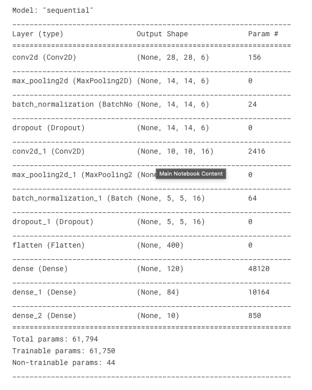
Defining the model strcture
#Model Definition
digit_model = models.Sequential()
#First Layer 6 kernels of size 5,5
digit_model.add(layers.Conv2D(6,(5,5), input_shape = (28,28,1), activation = 'relu', padding = "same"))
#max pooling with poolind size 2,2
digit_model.add(layers.MaxPooling2D(pool_size = (2,2)))
#Adding Batch Normalization
digit_model.add(layers.BatchNormalization())
#Dropout
digit_model.add(layers.Dropout(0.1))
#Second Layer 16 kernels of 5,5
digit_model.add(layers.Conv2D(16,(5,5), activation = 'relu'))
#Pooling
digit_model.add(layers.MaxPooling2D(2,2))
#Batch Norm
digit_model.add(layers.BatchNormalization())
#Dropout
digit_model.add(layers.Dropout(0.3))
#Flattening
digit_model.add(layers.Flatten())
#NN with 120-84-10 layers
digit_model.add(layers.Dense(120, activation='relu'))
digit_model.add(layers.Dense(84, activation='relu'))
digit_model.add(layers.Dense(10, activation = "softmax"))

#Model Summary
digit_model.summary()
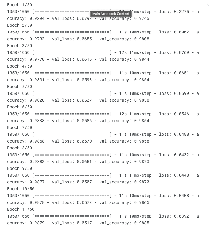
Model training
#Training the Model with Early Stopping with patience for 5 epochs.
callback = tf.keras.callbacks.EarlyStopping(monitor='accuracy',patience=5)
digit_model.compile(optimizer = "rmsprop",loss = tf.keras.losses.categorical_crossentropy, metrics=["accuracy"])

#Model Fit
LeNet_mod = digit_model.fit(epochs = 50, x = x_train, y= y_train,  verbose = 1, validation_data=(x_val,y_val),callbacks=callback)
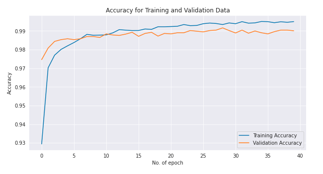
Accuracy
plt.figure(figsize=(10,5))
plt.plot(LeNet_mod.history["accuracy"], label = "Training Accuracy")
plt.plot(LeNet_mod.history["val_accuracy"], label = "Validation Accuracy");
plt.title('Accuracy for Training and Validation Data')
plt.ylabel('Accuracy')
plt.xlabel('No. of epoch')
plt.legend(loc = "lower right");
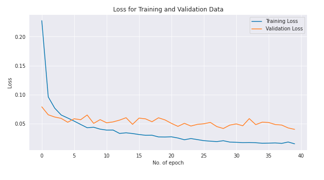
Loss
#Loss
plt.figure(figsize=(10,5))
plt.plot(LeNet_mod.history["loss"], label = "Training Loss")
plt.plot(LeNet_mod.history["val_loss"], label = "Validation Loss");
plt.title('Loss for Training and Validation Data')
plt.ylabel('Loss')
plt.xlabel('No. of epoch')
plt.legend(loc = "upper right");
Final Prediction
prediction = np.argmax(digit_model.predict(test), axis=-1)
#Generating Index
Imageid = [i for i in range(1,28000+1)]
#Creating data frame
d = {"ImageId":Imageid,"Label":prediction}
pred_df = pd.DataFrame(d)
pred_df.index = pred_df["ImageId"]
pred_df.drop("ImageId",axis=1,inplace=True)
pred_df.head()
pred_df.to_csv("/kaggle/working/sample_submission.csv",index=False)